Category Archives: explainer

Review of Fortune’s Formula by William Poundstone: The stranger-than-fiction tale of how to invest

What is a better investment objective?

  1. Grow as wealthy as possible as quickly as possible, or
  2. Maximize expected wealth for a given time period and level of risk

The question is at the heart of a fight between computer scientists and economists chronicled beautifully in the book Fortune’s Formula by Pulitzer Prize nominee William Poundstone. (See also David Pogue’s excellent review.*) From the book’s sprawling cast — Claude Shannon, Rudy Giuliani, Michael Milken, mobsters, and mob-backed companies (including what is now Time Warner!) — emerges an unlikely duel. Our hero, mathematician turned professional gambler and investor Edward Thorp, leads the computer scientists and information theorists preaching and, more importantly, practicing objective #1. Nobel laureate Paul Samuelson (who, sadly, recently passed away) serves as lead villain (and, to an extent, comic foil) among economists promoting objective #2 in often patronizing terms. The debate sank to surprisingly depths of immaturity, hitting bottom when Samuelson published an economist-peer-reviewed article written entirely in one-syllable words, presumably to ensure that his thrashing of objective #1 could be understood by even its nincompoop proponents.

Objective #1 — The Kelly criterion

Objective #1 is the have-your-cake-and-eat-it-too promise of the Kelly criterion, a money management formula first worked out by Bernoulli in 1738 and later rediscovered and improved by Bell Labs scientist John Kelly, proving a direct connection between Shannon-optimal communication and optimal gambling. Objective #1 matches common sense: who wouldn’t want to maximize growth of wealth? Thorp, college professor by day and insanely successful money manager by night, is almost certainly the greatest living example of the Kelly criterion at work. His track record is hard to refute.

If two twins with equal wealth invest long enough, the Kelly twin will finish richer with 100% certainty.

The Kelly criterion dictates exactly what fraction of wealth to wager on any available gamble. First consider a binary gamble that, if correct, pays $x for every $1 risked. You estimate that the probability of winning is p. As Poundstone states it, the Kelly rule says to invest a fraction of your wealth equal to edge/odds, where edge is the expected return per $1 and odds is the payoff per $1. Substituting, edge/odds = (x*p – 1*(1-p))/x. If the expected return is zero or negative, Kelly sensibly advises to stay away: don’t invest at all. If the expected return is positive, Kelly says to invest some fraction of your wealth proportional to how advantageous the bet is. To generalize beyond a single binary bet, we can use the fact that, as it happens, the Kelly criterion is entirely equivalent to (1) maximizing the logarithm of wealth, and (2) maximizing the geometric mean of gambles.

Investing according to the Kelly criterion achieves objective #1. The strategy provably maximizes the growth rate of wealth. Stated another way, it minimizes the time it takes to reach any given aspiration level, say $1 million, or your desired sized nest egg for retirement. If two twins with equal initial wealth were to invest long enough, one according to Kelly and the other not, the Kelly twin would finish richer with 100% certainty.

Objective #2

Objective #2 refers to standard economic dogma. Low-risk/high-return investments are always preferred to high-risk/low-return investments, but high-risk/high-return and low-risk/low-return are not comparable in general. Deciding between these is a personal choice, a function of the decision maker’s risk attitude. There is no optimal portfolio, only an efficient frontier of many Pareto optimal portfolios that trade off risk for return. The investor must first identify his utility function (how much he values a dollar at every level of wealth) in order to compute the best portfolio among the many valid choices. (In fact, objective #1 is a special case of #2 where utility for money is logarithmic. Deriving rather than choosing the best utility function is anathema to economists.)

Objective #2 is straightforward for making one choice for a fixed time horizon. Generalizing it to continuous investment over time requires intricate forecasting and optimization (which Samuelson published in his 1969 paper “Lifetime portfolio selection by dynamic stochastic programming”, claiming to finally put to rest the Kelly investing “fallacy” — p.210). The Kelly criterion is, astonishingly, a greedy (myopic) rule that at every moment only needs to worry about figuring the current optimal portfolio. It is already, by its definition, formulated for continuous investment over time.

Details and Caveats

There is a subtle and confusing aspect to objective #1 that took me some time and coaching from Sharad and Dan to wrap my head around. Even though Kelly investing maximizes long-term wealth with 100% certainty, it does not maximize expected wealth! The proof of objective #1 is a concentration bound that appeals to the law of large numbers. Wealth is, eventually, an essentially deterministic quantity. If a billion investors played non-Kelly strategies for long enough, then their average wealth might actually be higher than a Kelly investor’s wealth, but only a few individuals out of the billion would be ahead of Kelly. So, non-Kelly strategies can and will have higher expected wealth than Kelly, but with probability approaching zero. Note that, while Kelly does not maximize expected (average) wealth, it does maximize median wealth (p.216) and the mode of wealth. See Chapter 6 on “Gambling and Data Compression” (especially pages 159-162) in Thomas Cover’s book Elements of Information Theory for a good introduction and concise proof.

Objective #1 does have important caveats, leading to legitimate arguments against pure Kelly investing. First, it’s often too aggressive. Sure, Kelly guarantees you’ll come out ahead, but only if investing for “long enough”, a necessarily vague phrase that could mean, well, infinitely long. (In fact, a pure Kelly investor at any time has a 1 in n chance of losing all but 1/n of their wealth — p.229) The guarantee also only applies if your estimate of expected return per dollar is accurate, a dubious assumption. So, people often practice what is called fractional Kelly, or investing half or less of whatever the Kelly criterion says to invest. This admittedly starts down a slippery slope from objective #1 to objective #2, leaving the mathematical high ground of optimality to account for people’s distaste for risk. And, unlike objective #2, fractional Kelly does so in a non-principled way.

Even as Kelly investing is in some ways too aggressive, it is also too conservative, equating bankruptcy with death. A Kelly strategy will never risk even the most minuscule (measure zero) probability of losing all wealth. First, the very notion that each person’s wealth equals some precise number is inexact at best. People hold wealth in different forms and have access to credit of many types. Gamblers often apply Kelly to an arbitrary “casino budget” even though they’re an ATM machine away from replenishment. People can recover nicely from even multiple bankruptcies (see Donald Trump).

Some Conjectures

Objective #2 captures a fundamental trade off between expected return and variance of return. Objective #1 seems to capture a slightly different trade off, between expected return and probability of loss. Kelly investing walks the fine line between increasing expected return and reducing the long-run probability of falling below any threshold (say, below where you started). There are strategies with higher expected return but they end in ruin with 100% certainty. There are strategies with lower probability of loss but that grow wealth more slowly. In some sense, Kelly gets the highest expected return possible under the most minimal constraint: that the probability of catastrophic loss is not 100%. [Update 2010/09/09: The statements above are not correct, as pointed out to me by Lirong Xia. Some non-Kelly strategies can have higher expected return than Kelly and near-zero probability of ruin. But they will do worse than Kelly with probability approaching 1.]

It may be that the Kelly criterion can be couched in the language of computational complexity. Let Wt be your wealth at time t. Kelly investing grows expected wealth exponentially, something like E[Wt] = o(xt) for x>1. It simultaneously shrinks the probability of loss, something like Pr(Wt< T) = o(1/t). (Actually, I have no idea if the decay is linear: just a guess.) I suspect that relaxing the second condition would not lead to much higher expected growth, and perhaps that fractional Kelly offers additional safety without sacrificing too much growth. If formalized, this would be some sort of mixed Bayesian and worst-case argument. The first condition is a standard Bayesian one: maximize expected wealth. The second condition — ensuring that the probability of loss goes to zero — guarantees that even the worst case is not too bad.

Conclusions

Fortune’s Formula is vastly better researched than your typical popsci book: Poundstone extensively cites and quotes academic literature, going so far as to unearth insults and finger pointing buried in the footnotes of papers. Pounstone clearly understands the math and doesn’t shy away from it. Instead, he presents it in a detailed yet refreshingly accessible way, leveraging fantastic illustrations and analogies. For example, the figure and surrounding discussion on pages 197-201 paint an exceedingly clear picture of how objectives #1 and #2 compare and, moreover, how #1 “wins” in the end. There are other gems in the book, like

  • Kelly’s quote that “gambling and investing differ only by a minus sign” (p.75)
  • Louis Bachelier’s discovery of the efficient market hypothesis in 1900, a development that almost no one noticed until after his death (p.120)
  • Poundstone’s assertion that “economists do not generally pay much attention to non-economists” (p.211). The assertion rings true, though to be fair applies to most fields and I know many glaring exceptions.
  • The story of the 1998 collapse of Long-Term Capital Management and ensuing bailout is sadly amusing to read today (p.290). The factors are nearly identical to those leading to the econalypse of 2008: leverage + correlation + too big to fail. (Poundstone’s book was published in 2005.) Will we ever learn? (No.)

Fortune’s Formula is a fast, fun, fascinating, and instructive read. I highly recommend it.

__________
* See my bookmarks for other reviews of the book and some related research articles.

What is (and what good is) a combinatorial prediction market?

What exactly is a combinatorial prediction market?

2010 Update: Several of us at Yahoo! Labs, along with academic researchers, have theorized and written about combinatorial prediction markets for several years, as you’ll see below. But now we’ve gone beyond talking about them and actually built one. So the best way to answer the question is to see the market we built and play with it. It’s called Predictalot. The first version was based on the NCAA Men’s College Basketball tournament known as March Madness.

Combinatorial Madness

March Madness is the anything-can-happen-and-often-does tournament among the top 64 NCAA Men’s College Basketball teams. The “madness” of the games is rivaled only by the madness of fans competing to pick the winners. In Las Vegas, you can bet on many things, from individual games to the overall champion to more exotic “propositions” like which conference of teams will do best. Still, each gambling venue defines in advance exactly what you are allowed to bet on, offering an explicit list of usually no more than a few thousand choices.

A combinatorial market maker fulfills an almost magical promise: propose any obscure proposition, click “accept”, and your bet is placed: no doubt and no waiting.

In contrast, a combinatorial market could allow you to make up nearly any proposition you want on the fly, for example, “Duke will advance further than UNC” or “At least one of the top four seeds will lose in the first round”, or “ACC conference teams will win every game they play against lower-seeded SEC conference teams”. How many such propositions are there? Let’s count. There are 63 games (ignore the new play-in game), each of which could go to either to the favorite or the underdog, so there are 263 or over 9,220,000,000,000,000,000 (9.22 quintillion) outcomes, or ways the tournament in its entirety could unfold. Propositions are collections or sets of outcomes: for example “Duke will advance further than UNC” is a statement that’s true in something less than half of the 9.2 quintillion outcomes. Technically, then, there are 2263 possible propositions, a number that dwarfs the number of atoms in the universe. Clearly we could never write down a list that long, even inside a computer. However that doesn’t necessarily mean we can’t operate such a market if we are a little clever about how we implement it, as we’ll see below.

So here is my informal definition: a combinatorial market is one where users can construct their own bets by mixing and matching options in myriad ways, sort of like ordering a Wendy’s hamburger. (Or highly customized insurance.)

The Details

Now I’ll try for a more precise definition.

Just to set the vocabulary straight, outcomes are all possible things that might happen: for example all five candidates in an election, all 30 teams in an NBA Championship market, all 3,628,800 (or 10!) finish orderings in a ten-horse race, or all 9.2 quintillion March Madness tournament results. Among the outcomes, in the end one and only one of them will actually occur; traders try to predict which.

Bids express what outcome(s) traders think will happen. Bids also contain the risk-reward ratio the trader is willing to accept: the amount she wins if correct and the amount she is willing to lose if incorrect.

There are two reasons why we might call a market “combinatorial”: either the bids are combinatorial or the outcomes are combinatorial. The latter poses a much harder computational problem. I’ll start with the former.

  1. Combinatorial bids. A combinatorial bid or bundle bid is a concise expression representing a collection or set of outcomes, for example “a Western Conference team will win the NBA Championship”, encompassing 15 possible outcomes, or “horse A will finish ahead of horse B” in a ten-horse race, encoding 1,814,400, or half, of the possible outcomes. Yoopick, our experimental sports prediction market on Facebook, features a type of combinatorial bidding called interval bidding. Traders select the range they think the final score difference will fall into, for example “Pittsburgh will win by between 2 and 11 points”. An interval bet is actually a collection of bets on every outcome between the left and right endpoints of the range.

    For comparison, a non-combinatorial bid is a bet on a single outcome, for example “candidate O will win the election”. The vast majority of fielded prediction markets handle only non-combinatorial bids.

    What are examples of combinatorial bids besides Yoopick? Abe Othman built an interval betting interface similar to Yoopick (he came up with it on his own, proving that great minds think alike) to predict when the new CMU computer science building will finish construction. Additional examples include Bossaerts et al.’s concept of combined value trading and the parimutuel call market mechanism [Baron & Lange, Lange & Economides, Peters et al.]. 2010 Update: Predictalot is our latest example of a market featuring both combinatorial bids and outcomes.

  2. Combinatorial outcomes. The March Madness scenario is an example of combinatorial outcomes. The number of outcomes (e.g., 9.2 quintillion) may be so huge that we could never hope to track every outcome explicitly inside a computer. Instead, outcomes themselves are defined implicitly according to some counting process that involves enumerating every possible combination of base objects. For example, the outcome space could be all n! possible finish orderings of an n-horse race. Or all 2n combinations of n binary events. In both cases, the number of outcomes grows exponentially in the number of base objects n, quickly becoming unimaginably large as n grows.

    A market with combinatorial outcomes is almost nonsensical without allowing combinatorial bids as well, since individual outcomes are like microbes on a needle on a cruise ship of hay in a universe-sized sea. No one wants to bet on these minuscule possibilities one at a time. Instead, traders bet on high-level properties of outcomes, like “Duke will advance further than UNC”, that encode sets of outcomes. Here are some example forms of combinatorics and corresponding bidding languages that seem natural:

    • Boolean betting. Outcomes are combinations of binary events. Bids are phrased in Boolean logic. So if base objects are “Democrat will win in Alabama”, “Democrat will win in Alaska”, etc. for all fifty US states, and outcomes are all 250 possible ways the election might swing across all 50 states, then bids may be of the form “Democrat will win in Ohio and Florida, but not Virginia”, or “Democrat will win Nevada if they win California”, etc. For further reading, see Hanson’s paper on combinatorial market makers and our papers on the computational complexity of Boolean betting auctioneers and market makers.
    • Tournament betting. This is the March Madness example and a special case of Boolean betting. See our paper on tournament betting market makers.
    • Permutation betting. Outcomes are possible finish orderings in a horse race. Bids are properties of orderings, for example “Horse B will finish ahead of horse D”, or “Horse B will finish between 3rd and 7th place”. See our papers on permutation betting auctioneers and market makers.
    • Taxonomy betting. Base objects are (discretized) numbers arranged in a taxonomy, for example web site page views organized by topic, subtopic, etc. Outcomes are all possible combinations of the numbers. Bets can be placed on the range of any number in the taxonomy, for example page views of a sports web site, page views of the NBA subsection of the web site, etc. Coming soon: a paper on taxonomy betting led by Mingyu Guo at Duke. [Update: here is the paper.]

    We summarize some of these in a short article on Combinatorial betting and a more detailed book chapter on Computational aspects of prediction markets.

    2009 Update: Gregory Goth writes an excellent and accessible summary in the March 2009 Communcations of the ACM, p.13.

Auctioneer versus market maker

So far, I’ve only talked about the form of bids from traders. Next I’ll discuss the actual mechanics of the marketplace, or how bids are processed. How does the market operator decide which bids to accept or reject? At what prices?

I’ll focus on two major possibilities: either the market operator acts as an auctioneer or he acts as an automated market maker.

An auctioneer only matches up willing traders with each other — the auctioneer never takes on any risk of his own. This is how most financial exchanges like the stock market operate, and how intrade and betfair operate. (A call market is a special case where the auctioneer collects many bids over a period of time, then processes them all together in a single batch.)

An automated market maker will quote a price for any bet whatsoever. Even lone traders can place their bet with the market maker as long as they accept the price, greatly enhancing liquidity. The liquidity comes at a cost though: an automated market maker can and often does lose money, though clever pricing algorithms can guarantee that losses won’t mount beyond a fixed amount set in advance. Hanson’s logarithmic market scoring rule market maker is far and away the most popular for prediction markets, and for good reason: it’s simple, has nice modularity properties, and behaves well in practice. We catalog a number of bounded-loss market makers in this paper. The dynamic parimutuel market used in the (now closed) Yahoo! Tech Buzz Game can be thought of as another type of automated market maker.

A market with combinatorial outcomes almost requires a market maker to function smoothly. When traders have such a mind-boggling array of choices, the chances that two or more of their bets will exactly counter each other seems remote. If trades are rarely filled, then traders won’t bother bidding at all, causing a no-chicken-no-egg spiral into failure.

One the other hand, a market maker allows anyone to get a price quote at any time on any bet, no matter how convoluted or specific, even if no other traders had thought about that particular possibility. Thus interacting with a combinatorial market maker can be highly satisfying: propose any obscure proposition, click “accept price”, and your bet is placed: no doubt and no waiting.

I’ll discuss one more technicality. An auctioneer must decide whether bids can be partially filled, giving traders both less risk and less reward than they requested, in the same ratio. This makes sense. If I’m willing to risk $100 to win $200, I’d almost surely risk $50 to win $100 instead. Allowing partial fills greatly simplifies life for the auctioneer too. If bids are divisible, or can be filled in part, the auctioneer can use efficient linear programming algorithms; if bids are indivisible, the auctioneer must use integer programming algorithms that may be intractable. For more on the divisible/indivisible distinction, see Bossaerts et al. and Fortnow et al. Allowing divisible bids seems the logical choice in most scenarios, since the market functions better and most traders won’t mind.

The benefits of combinatorial markets

Why do we need or want combinatorial markets? Simply put, they allow for the collection of more information, the life-blood of every prediction market. Combinatorial outcomes allow traders to assess the correlations among base objects, not just their independent likelihoods, for example the correlation between Democrats winning in Ohio and Pennsylvania. Understanding correlations is key in many applications, including risk assessment: one might argue that the recent financial meltdown is partly attributable to an underestimation of correlation among firms and securities and the chances of cascading failures.

Although financial and betting exchanges, bookmakers, and racetracks are modernizing, turning their operations over to computers and moving online, their core logic for processing bids hasn’t changed much since auctioneers were people. For simplicity, they treat all bets like apples and oranges, processing them independently, even when they are more like hamburgers and cheeseburgers. For example, bets on a horse “to win” and “to finish in the top two” are managed separately at the racetrack, as are options to buy a stock at “strike price 30” and “strike price 20” on the CBOE. In both cases it’s a logical truism that the first is worth less than the second, yet the market pleads ignorance, leaving it to traders to enforce consistent pricing.

In a combinatorial market, a bet on “Duke will win the tournament” automatically increases the odds on “Duke will win in the first round”, as it logically should. Mindless mechanical tasks like this are handled automatically, by algorithms that are far better at it anyway, freeing up traders for the primary task a prediction market asks them to do: provide information. Traders are free to express their information in whatever form they find most natural, and it all flows into the same pool of liquidity.

I discuss the benefits of combinatorial bids further in this post, including one benefit I don’t mention here: smarter accounting, or making sure no more is reserved from a trader’s balance than necessary to cover their worst-case loss.

The disadvantages of combinatorial markets

I would argue that there is virtually no disadvantage to allowing combinatorial bids. They are more flexible and natural for traders, and they eliminate redundancy and thus concentrate liquidity (again I refer the reader to this previous post). Allowing indivisible combinatorial bids can cause computational problems, but as I argue above, divisible bids make more sense anyway.

On the other hand, there can be disadvantages to markets with combinatorial outcomes. First, trader attention and liquidity may be severely fractured, since there are nearly limitless things to bet on.

Second, and perhaps more troublesome, running an auctioneer with combinatorial outcomes is computationally intractable (specifically, NP-hard, or as hard as solving SAT) and running a market maker is even harder (specifically, #P-hard, as hard as counting SAT), meaning that the amount of time needed to run is proportional to the number of outcomes, exponential in the number of objects.

It gets worse. Even if we place strict limits on what types of bets traders can make, the market may still be infeasible to run. For example, even if all bets are pairwise, like “Horse B will finish ahead of horse D”, the auctioneer and market maker problems for permutation betting remain NP-hard and #P-hard, respectively. Likewise, Boolean betting remains hard even if the most complicated bet allowed is joining two events, like “E will happen and F will not” [see Chen et al. and Fortnow et al.].

How to build one

Now for some good news: in some cases, fast algorithms are possible. If all bets are subset bets of the form “Horse A will finish in position 1,2, or 10” or “Horse B,C, or E will finish in position 3”, then permutation betting with an auctioneer is feasible (using a combination of linear programming and maximum matching), even though the corresponding market maker problem is #P-hard. If all bets are of the form “Team B will advance to round k”, tournament betting with a market maker is feasible (using Bayesian network inference). Taxonomy betting with a market maker is feasible (using dynamic programming).

Finally, even better news: fast market maker approximation algorithms are not only possible and practical, they work without limiting what people can bet on, fulfilling the almost magical promise I made at the outset of constructing any bet you can imagine on the fly. Approximation works because people like to bet on things that have a decent chance of happening, say between a 1% and 99% chance. Standard sampling algorithms, including importance sampling and MCMC, are good at approximating prices for such reasonable events. For the extreme (e.g., 1-in-a-billion) events, sampling may fail, so the market maker will have to round off in its own favor to be safe.

Wrapping up, in my mind, the best way to implement a combinatorial-outcome prediction market is as follows:

  • Use a market maker. Without one, traders are unlikely to find each other in the sea of choices. Specifically, use Hanson’s LMSR market maker.
  • Use an approximation algorithm for pricing. Importance sampling seems to work well. MCMC is another possibility. See Appendix A of this paper.
  • The interface is absolutely key, and the aspect I’m least qualified to opine on. I think Predictalot, WeatherBill, Yoopick, and WhenWillWeMove point in the right direction.

2010 Update: Predictalot is our first pass at carrying through on this vision of how to build a combinatorial prediction market. In building it, we learned a great deal already, for example that sampling is much much trickier than I had initially imagined, and that it’s easy to accidentally create arbitrage loopholes if you’re not extremely careful with the math.

I glossed over a number of details. For example, care must be taken for the market maker to always round approximations in its own favor to avoid opening itself up to arbitrage attacks. Another difficulty is how to implement smart accounting to allow traders maximum leverage when they place many interrelated bets. The assumption that traders could lose all their bets is far too conservative — they might have bets that provably cannot simultaneously lose — but may serve as a reasonable starting point in practice.

The right way to implement a multi-outcome prediction market: Linear programming

There are many examples of multi-outcome prediction markets, for example election markets with more than two candidates, or sports championship markets with dozens of teams.

What is the best way to implement a multi-outcome prediction market?

The simplest way is to effectively ignore the fact that there are multiple outcomes, breaking up the market into a bunch of separate binary markets, one for each outcome. Each outcome-market is an independent instrument with its own order flow and processing.

This seems to be the most common approach, taken by for example intrade, IEM, racetracks, and most financial exchanges. IMHO, it’s the wrong way, for three reasons.

  1. Splitting up a market can hurt liquidity. In a split market, there are effectively two ways to do everything (e.g., buy outcome 1 equals sell outcomes 2 through N), so traders may not see the best price for what they want to do, and orders may not fill at the best price available. There may even be orders that together constitute an agreeable trade, yet are stuck waiting in separate queues.
  2. A split market may also slow information propagation. Price changes in one outcome do not directly affect prices of other outcomes; it’s left to arbitrageurs to propagate logical implications.
  3. Finally, a naïve implementation of a split market may limit traders’ leverage, forcing them set aside more money than necessary to complete a set of trades. For example, on IEM, short selling one share at $0.99 requires that you have $1 in your account, even though the most you could possibly lose in this transaction is $0.01. The reason is that to short sell on IEM you must first buy the bundle of all outcomes for $1, then sell off the outcome that you don’t want.

IEM has possibly the worst implementation, suffering from all three problems.

Intrade’s implementation is slightly better: they at least handle leverage correctly.

Newsfutures is smarter still.1 They generate phantom bids to reflect the redundant ways to place bets. For example, if there are bids for outcomes 2 through N that add up to $0.80, they place a phantom ask on outcome 1 for $0.20. A trader who accepts the ask, buying outcome 1 for $0.20, actually sells outcomes 2 through N behind the scenes, an entirely equivalent transaction. Chris Hibbert has a more elaborate methodology for eking out as much liquidity as possibly using phantom bids, an approach he has implemented plans to implement in his Zocalo platform.

Yet phantom bids are a band-aid that cannot entirely heal a fractured market. Still missing is the ability to trade bundles of outcomes in a single transaction.

For example, consider the US National Basketball Association championship market, with 30 teams. A split market (possibly with phantom bids) works great for betting on individual teams one at a time, but is terribly cumbersome for betting on groups of teams. For example, betting that a Western conference team will win requires 15 separate transactions. A common fix is to open yet another market in each popular bundle, however this limits choice and exacerbates all three problems above.

Bundling is especially useful with interval bets. For example, consider this bet on the peak price of gasoline through September 2008, broken up into intervals $3-$3.25, $3.25-$3.40, etc. In order to bet that gas prices will peak between, say, $3.40 and $4.30, you must buy all six outcomes spanning the interval, one at a time. (Moreover, you must sum the six outcome prices manually to compute a price quote.)

Fortunately, there is a trading engine that solves all three problems above and also allows bundle bets…

It’s linear programming!

Bossaerts et al. call it combined value trading. Baron & Lange, Lange & Economides and Peters et al. call it a parimutuel call market. Fortnow et al. and Chen et al. describe it in the context of combinatorial call markets.

Whatever you call it, the underlying principle is relatively straightforward, and it seems inherently the right way to implement a multi-outcome market. Yet I’ve rarely seen it done. The only example I know of is the now defunct economic derivatives markets run by Longitude, Goldman Sachs, and Deutsche Bank.

The set up of the linear program is as follows. Each order is associated with a decision variable x that ranges between 0 and 1, encoding the fraction of the order that the auctioneer can accept.2 There is one constraint per outcome that ensures that the auctioneer never loses money across all outcomes. The choice of objective function depends on the auctioneer’s goals, but something like maximizing the fill fraction makes sense.

Once the program is set up, the auctioneer solves for the x variables to determine which orders to accept in full (x=1), which to accept partially (0<x<1), and which to reject (x=0). The program can be solved either in batch mode, after waiting to collect a number of orders, or in continuous mode immediately as new orders arrive. Batch mode corresponds to a call market. Continuous mode corresponds to a continuous auction, a generalization of the continuous double auction mechanism of the stock market.

Each order consists of a price, a quantity, and an outcome bundle. Traders can just as easily bet on single outcomes, negations of outcomes, or sets of outcomes (e.g., all Western Conference NBA teams). Every order goes into the same pool of liquidity no matter how it is phrased.

Price quotes are queries to the linear program of the form “at what price p will this order be accepted in full?” (I believe that bounds on the dual variables of the LP can be interpreted as bid and ask price quotes.)

Lange & Economides and Peters et al. devise clever ways to make prices unique rather than bid-ask ranges, by injected a small subsidy to seed the market at the onset.

Note that Hanson’s market scoring rules market maker also elegantly solves all the same problems as the LP formulation, including handling bundle bets. However, the market maker requires a patron to subsidize the market, while the LP auctioneer formulation is budget balanced — that is, can never lose money.

Also note that I am not talking about a combinatorial-outcome market here. In this post, I am imagining that the number of outcomes is tractable — small enough so that we can explicitly list, store, and compute across all of the outcomes. A true combinatorial-outcome market, on the other hand, has an exponentially large number of outcomes making it impossible to even list them all explicitly, and forcing all calculations to operate on an implicit representation of outcomes, for example Boolean combinations of base events.

1Apparently worked out in conjunction with Brian Galebach, a mathematician and Newsfutures fan extraordinaire who runs the prediction contest probabilitysports.com.
2Alternatively, the variables can range between 0 and q, where q is the quantity of shares ordered.

The wisdom of the ProbabilitySports crowd

One of the purest and most fascinating examples of the “wisdom of crowds” in action comes courtesy of a unique online contest called ProbabilitySports run by mathematician Brian Galebach.

In the contest, each participant states how likely she thinks it is that a team will win a particular sporting event. For example, one contestant may give the Steelers a 62% chance of defeating the Seahawks on a given day; another may say that the Steelers have only a 44% chance of winning. Thousands of contestants give probability judgments for hundreds of events: for example, in 2004, 2,231 ProbabilityFootball participants each recorded probabilities for 267 US NFL Football games (15-16 games a week for 17 weeks).

An important aspect of the contest is that participants earn points according to the quadratic scoring rule, a scoring method designed to reward accurate probability judgments (participants maximize their expected score by reporting their best probability judgments). This makes ProbabilitySports one of the largest collections of incentivized1 probability judgments, an extremely interesting and valuable dataset from a research perspective.

The first striking aspect of this dataset is that most individual participants are very poor predictors. In 2004, the best score was 3747. Yet the average score was an abysmal -944 points, and the median score was -275. In fact, 1,298 out of 2,231 participants scored below zero. To put this in perspective, a hypothetical participant who does no work and always records the default prediction of “50% chance” for every team receives a score of 0. Almost 60% of the participants actually did worse than this by trying to be clever.

ProbabilitySports participants' calibration
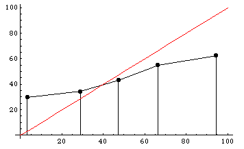
Participants are also poorly calibrated. To the right is a histogram dividing participants’ predictions into five regions: 0-20%, 20-40%, 40-60%, 60-80%, and 80-100%. The y-axis shows the actual winning percentages of NFL teams within each region. Calibrated predictions would fall roughly along the x=y diagonal line, shown in red. As you can see, participants tended to voice much more extreme predictions than they should have: teams that they said had a less than 20% chance of winning actually won almost 30% of the time, and teams that they said had a greater than 80% chance of winning actually won only about 60% of the time.

Yet something astonishing happens when we average together all of these participants’ poor and miscalibrated predictions. The “average predictor”, who simply reports the average of everyone else’s predictions as its own prediction, scores 3371 points, good enough to finish in 7th place out of 2,231 participants! (A similar effect can be seen in the 2003 ProbabilityFootball dataset as reported by Chen et al. and Servan-Schreiber et al.)

Even when we average together the very worst participants — those participants who actually scored below zero in the contest — the resulting predictions are amazingly good. This “average of bad predictors” scores an incredible 2717 points (ranking in 62nd place overall), far outstripping any of the individuals contributing to the average (the best of whom finished in 934th place), prompting someone in this audience to call the effect the “wisdom of fools”. The only explanation is that, although all these individuals are clearly prone to error, somehow their errors are roughly independent and so cancel each other out when averaged together.

Daniel Reeves and I follow up with a companion post on Robin Hanson’s OvercomingBias forum with some advice on how predictors can improve their probability judgments by averaging their own estimates with one or more others’ estimates.

In a related paper, Dani et al. search for an aggregation algorithm that reliably outperforms the simple average, with modest success.

     1Actually the incentives aren’t quite ideal even in the ProbabilitySports contest, because only the top few competitors at the end of each week and each season win prizes. Participants’ optimal strategy in this all-or-nothing type of contest is not to maximize their expected score, but rather to maximize their expected prize money, a subtle but real difference that tends to induce greater risk taking, as Steven Levitt describes well. (It doesn’t matter whether participants finish in last place or just behind the winners, so anyone within striking distance might as well risk a huge drop in score for a small chance of vaulting into one of the winning positions.) Nonetheless, Wolfers and Zitzewitz show that, given the ProbabilitySports contest setup, maximizing expected prize money instead of expected score leads to only about a 1% difference in participants’ optimal probability reports.

Evaluating probabilistic predictions

A number of naysayers [Daily Kos, The Register, The Big Picture, Reason] are discrediting prediction markets, latching onto the fact that markets like TradeSports and NewsFutures failed to call this year’s Democratic takeover of the US Senate. Their critiques reflect a clear misunderstanding of the nature of probabilistic predictions, as many others [Emile, Lance] have pointed out. Their misunderstanding is perhaps not so surprising. Evaluating probabilistic predictions is a subtle and complex endeavor, and in fact there is no absolute right way to do it. This fact may pose a barrier for the average person to understand and trust (probabilistic) prediction market forecasts.

In an excellent article in The New Republic Online [full text], Bo Cowgill and Cass Sunstein describe in clear and straightforward language the fallacy that many people seem to have made, interpreting a probabilistic prediction like “Democrats have a 25% chance of winning the Senate” as a categorical prediction “The Democrats will not win the Senate”. Cowgill and Sunstein explain the right way to interpret probabilistic predictions:

If you look at the set of outcomes estimated to be 80 percent likely, about 80 percent of them [should happen]; events estimated to be 70 percent likely [should] happen about 70 percent of the time; and so on. This is what it means to say that prediction markets supply accurate probabilities.

Technically, what Cowgill and Sunstein describe is called the calibration test. The truth is that the calibration test is a necessary test of prediction accuracy, but not a sufficient test. In other words, for a predictor to be considered good it must pass the calibration test, but at the same time some very poor or useless predictors may also pass the calibration test. Often a stronger test is needed to truly evaluate the accuracy of probabilistic predictions.

For example, suppose that a meteorologist predicts the probability of rain every day. Now suppose this meteorologist is lazy and he predicts the same probability every day: he simply predicts the annual average frequency of rain in his location. He doesn’t ever look at cloud cover, temperature, satellite imagery, computer models, or even whether it rained the day before. Clearly, this meteorologist’s predictions would be uninformative and nearly useless. However, over the course of a year, this meteorologist would perform very well according to the calibration test. Assume it rains on average 10% of the time in the meteorologist’s city, so he predicts “10% chance” every day. If we test his calibration, we find that, among all the days he predicted a 10% chance of rain (i.e., every day), it actually rained about 10% of the time. This lazy meteorologist would get a nearly perfect score according to the calibration test. A hypothetical competing meteorologist who actually works hard to consider all variables and evidence, and who thus predicts different percentages on different days, could do no better in terms of calibration.

The above example suggests that good predictions are not just well calibrated: good predictions are, in some sense, both variable AND well calibrated. So what is the “right” way to evaluate probabilistic predictions? There is no single absolute best way, though several tests are appropriate, and probably can be considered stronger tests than the calibration test. In our paper “Does Money Matter?” we use four evaluation metrics:

  1. Absolute error: The average over many events of lose_PR, the probability assigned to the losing outcome(s)
  2. Mean squared error: The square root of the average of (lose_PR)2
  3. Quadratic score: The average of 100 – 400*(lose_PR)2
  4. Logarithmic score: The average of log(win_PR), where win_PR is the probability assigned to the winning outcome

Note that the absolute value of these metrics is not very meaningful. The metrics are useful only when comparing one predictor against another (e.g., a market against an expert).

My personal favorite (advocated in papers and presentations) is the logarithmic score. The logarithmic score is one of a family of so-called proper scoring rules designed so that an expert maximizes her expected score by truthfully reporting her probability judgment (the quadratic score is also a proper scoring rule). Stated another way, experts with more accurate probability judgments should be expected to accumulate higher scores on average. The logarithmic score is closely related to entropy: the negative of the logarithmic score gives the amount (in bits of information) that the expert is “surprised” by the actual outcome. Increases in logarithmic score can literally be interpreted as measuring information flow.

Actually, the task of evaluating probabilistic predictions is even trickier than I’ve described. Above, I said that a good predictor must at the very least pass the calibration test. Actually, that’s only true when the predicted events are statistically independent. It is possible for a perfectly valid predictor to appear miscalibrated when the events he or she is predicting are highly correlated, as discussed in a previous post.

Implementing Hanson's Market Maker

Robin Hanson invented a wonderful market maker well suited for use in prediction market applications with a long name: the logarithmic market scoring rule market maker, which I’ll abbreviate as LMSR. (In fact, Hanson invented an entire class of market scoring rule market makers, but the logarithmic variant seems the most useful.) Hanson’s two papers on the subject are excellent, but Hanson does not spend a lot of time explaining how LMSR functions as a market maker in the typical sense. Instead, Hanson mostly emphasizes a second, alternate way of thinking about his market maker, as a “sequential shared scoring rule”, which I will not try to explain here. Hanson prefers to describe trader behavior in terms of “changing the price” instead of “buying and selling shares”. In my opinion, most people who encounter LMSR for the first time don’t quite see how beautifully and naturally LSMR can be used as a market maker in a standard prediction market setting. In fact, I am embarrassed to admit that upon my own first reading of Hanson’s papers, I did not fully “get it”. It took my seeing LMSR implemented in practice, by Todd Proebsting at Microsoft Research for Microsoft’s internal prediction markets, to realize how elegantly LMSR can be used as a market maker in an otherwise typical prediction market. LMSR is now being used in several places, including an implementation at InklingMarkets with a wonderfully intuitive interface, the Washington Stock Exchange, BizPredict, and (reportedly) at YooNew. Net Exchange was one of the first to use LMSR, though they seem to favor Hanson’s “change the price” interface over the more widespread “buy and sell shares” interface. As Chris Masse is quick to point out, LMSR has achieved much more widespread use than my own competing invention, the dynamic parimutuel market maker, which so far is being used in only one place: our own Yahoo! Tech Buzz Game.

In this post I will try to explain how to implement LMSR in a way that I believe most people familiar with prediction markets will understand. This interpretation of LMSR is not new: it’s the way Proebsting thinks about LMSR and it’s implicit “between the lines” in Hanson’s papers. But I haven’t seen this interpretation of LMSR written up anywhere, so I’m hoping that others can benefit from this explanation. The following understanding of LMSR was developed over the past few months together with my colleague Yiling Chen.

Suppose there are two outcomes that traders can buy or sell shares of (bet on or against) such that one and only one of the two outcomes is guaranteed to eventually occur. For example, the two outcomes could be “a Democrat wins the 2008 US Presidential election” and “a Democrat does not win the 2008 US Presidential election”. Each share is worth exactly $1 if and only if the trader is correct. In other words, one share of “Democrat wins” pays $1 if, in 2008, a Democrat actually wins the election, and is worthless otherwise. The following description can be easily generalized to any number of (disjoint and exhaustive) outcomes, including the case of combinatorial markets, but for ease of exposition I’ll stick to the two-outcome case.

The market maker keeps track of how many shares have been purchased by traders in total so far for each outcome: that is, the number of shares outstanding for each outcome. Let q1 and q2 be the number (“quantity”) of shares outstanding for each of the two outcomes. The market maker also maintains a cost function C(q1,q2) which records how much money traders have collectively spent so far, and depends only on the number of shares outstanding, q1 and q2. For LMSR, the cost function is:

C = b * ln(eq1/b+eq2/b)

where “ln” is the natural logarithm function, “e” is the constant e=2.718…, and “b” is a parameter that the market maker must choose. The parameter “b” controls the maximum possible amount of money the market maker can lose (which happens to be b*ln2 in the two-outcome case). The larger “b” is, the more money the market maker can lose. But a larger “b” also means the market has more liquidity or depth, meaning that traders can buy more shares at or near the current price without causing massive price swings.

Traders arrive one at a time and tell the market maker how many shares they want to buy or sell of each outcome. Traders say, for example, “I want to buy 13 shares of outcome 1 — how much will that cost?”, or “I want to sell 250 shares of outcome 2 — how much will you pay me?”. The market maker uses the cost function to answer these questions. The cost to buy 13 shares of outcome 1 is simply C(q1+13,q2) – C(q1,q2). The “cost” to sell 250 shares of outcome 2 is C(q1,q2-250) – C(q1,q2), which will be a negative number (negative cost), meaning that the seller receives money in return for the shares. In general, if a trader wants to buy or sell shares of either or both outcomes so as to change the number of shares outstanding from (q1,q2) to (q1*,q2*), then he or she must pay C(q1*,q2*) – C(q1,q2) dollars. If this amount is negative it means the trader receives money instead of paying money.

Here’s a simple example. Suppose b=100 and no one has purchased any shares yet, so q1=q2=0. A trader arrives who wants to buy 10 shares of outcome 1. The trader must pay:

C(10,0)-C(0,0) = 100 * ln(e10/100+e0) – 100 * ln(e0+e0) = $5.12

Now suppose that at some time later, the number of shares outstanding for outcome 1 is q1=50 and the number of shares outstanding of outcome 2 is q2=10. Now the same trader above returns to the market and wants to sell her 10 shares. The trader’s “payment” is:

C(40,10)-C(50,10) = 100 * ln(e40/100+e10/100) – 100 * ln(e50/100+e10/100) = -$5.87

This is a negative number so it means the trader receives $5.87. So in the end the trader made a round-trip profit of $0.75.

That’s it! Well, almost. If the market maker wants to quote a “current price”, he can. The current price for outcome 1 is:

price1 = eq1/b/(eq1/b+eq2/b)

and similarly for price2. But note that the current price only applies for buying a miniscule (infinitesimal, in fact) number of shares. As soon as a trader starts buying, the price immediately starts going up. In order to figure out the total cost for buying some number of shares, we should use the cost function C, not the price function. (If you remember your calculus: The total cost for buying k of shares of outcome 1 is the integral of the price function from q1 to q1+k. The price function (“price1”) is the derivative of the cost function C with respect to q1, and the cost function is the integral of the price function.)

Finally, although I won’t go into the details here, one can generalize the above so that the market maker can handle limit orders, for example an order to “buy up to 100 shares of outcome 1, each at price less than or equal to $0.80”. But if unfilled limit orders like this are allowed to persist, the market maker logic can get a little complicated.

As I mentioned, Hanson actually invented an entire class of market makers: he shows how to turn any proper scoring rule into a market maker. Yiling Chen and I have derived the cost and price functions corresponding to the quadratic scoring rule. It turns out, however, that the quadratic scoring rule market maker is not very interesting or useful in practice. I’ll save the details for another day. We’re also working on additional classes of market makers that do seem useful, results we hope to report on soon [update: see our paper “A utility framework for bounded-loss market makers”].