Category Archives: research

The wisdom of the ProbabilitySports crowd

One of the purest and most fascinating examples of the “wisdom of crowds” in action comes courtesy of a unique online contest called ProbabilitySports run by mathematician Brian Galebach.

In the contest, each participant states how likely she thinks it is that a team will win a particular sporting event. For example, one contestant may give the Steelers a 62% chance of defeating the Seahawks on a given day; another may say that the Steelers have only a 44% chance of winning. Thousands of contestants give probability judgments for hundreds of events: for example, in 2004, 2,231 ProbabilityFootball participants each recorded probabilities for 267 US NFL Football games (15-16 games a week for 17 weeks).

An important aspect of the contest is that participants earn points according to the quadratic scoring rule, a scoring method designed to reward accurate probability judgments (participants maximize their expected score by reporting their best probability judgments). This makes ProbabilitySports one of the largest collections of incentivized1 probability judgments, an extremely interesting and valuable dataset from a research perspective.

The first striking aspect of this dataset is that most individual participants are very poor predictors. In 2004, the best score was 3747. Yet the average score was an abysmal -944 points, and the median score was -275. In fact, 1,298 out of 2,231 participants scored below zero. To put this in perspective, a hypothetical participant who does no work and always records the default prediction of “50% chance” for every team receives a score of 0. Almost 60% of the participants actually did worse than this by trying to be clever.

ProbabilitySports participants' calibration
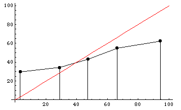
Participants are also poorly calibrated. To the right is a histogram dividing participants’ predictions into five regions: 0-20%, 20-40%, 40-60%, 60-80%, and 80-100%. The y-axis shows the actual winning percentages of NFL teams within each region. Calibrated predictions would fall roughly along the x=y diagonal line, shown in red. As you can see, participants tended to voice much more extreme predictions than they should have: teams that they said had a less than 20% chance of winning actually won almost 30% of the time, and teams that they said had a greater than 80% chance of winning actually won only about 60% of the time.

Yet something astonishing happens when we average together all of these participants’ poor and miscalibrated predictions. The “average predictor”, who simply reports the average of everyone else’s predictions as its own prediction, scores 3371 points, good enough to finish in 7th place out of 2,231 participants! (A similar effect can be seen in the 2003 ProbabilityFootball dataset as reported by Chen et al. and Servan-Schreiber et al.)

Even when we average together the very worst participants — those participants who actually scored below zero in the contest — the resulting predictions are amazingly good. This “average of bad predictors” scores an incredible 2717 points (ranking in 62nd place overall), far outstripping any of the individuals contributing to the average (the best of whom finished in 934th place), prompting someone in this audience to call the effect the “wisdom of fools”. The only explanation is that, although all these individuals are clearly prone to error, somehow their errors are roughly independent and so cancel each other out when averaged together.

Daniel Reeves and I follow up with a companion post on Robin Hanson’s OvercomingBias forum with some advice on how predictors can improve their probability judgments by averaging their own estimates with one or more others’ estimates.

In a related paper, Dani et al. search for an aggregation algorithm that reliably outperforms the simple average, with modest success.

     1Actually the incentives aren’t quite ideal even in the ProbabilitySports contest, because only the top few competitors at the end of each week and each season win prizes. Participants’ optimal strategy in this all-or-nothing type of contest is not to maximize their expected score, but rather to maximize their expected prize money, a subtle but real difference that tends to induce greater risk taking, as Steven Levitt describes well. (It doesn’t matter whether participants finish in last place or just behind the winners, so anyone within striking distance might as well risk a huge drop in score for a small chance of vaulting into one of the winning positions.) Nonetheless, Wolfers and Zitzewitz show that, given the ProbabilitySports contest setup, maximizing expected prize money instead of expected score leads to only about a 1% difference in participants’ optimal probability reports.

Implementing Hanson's Market Maker

Robin Hanson invented a wonderful market maker well suited for use in prediction market applications with a long name: the logarithmic market scoring rule market maker, which I’ll abbreviate as LMSR. (In fact, Hanson invented an entire class of market scoring rule market makers, but the logarithmic variant seems the most useful.) Hanson’s two papers on the subject are excellent, but Hanson does not spend a lot of time explaining how LMSR functions as a market maker in the typical sense. Instead, Hanson mostly emphasizes a second, alternate way of thinking about his market maker, as a “sequential shared scoring rule”, which I will not try to explain here. Hanson prefers to describe trader behavior in terms of “changing the price” instead of “buying and selling shares”. In my opinion, most people who encounter LMSR for the first time don’t quite see how beautifully and naturally LSMR can be used as a market maker in a standard prediction market setting. In fact, I am embarrassed to admit that upon my own first reading of Hanson’s papers, I did not fully “get it”. It took my seeing LMSR implemented in practice, by Todd Proebsting at Microsoft Research for Microsoft’s internal prediction markets, to realize how elegantly LMSR can be used as a market maker in an otherwise typical prediction market. LMSR is now being used in several places, including an implementation at InklingMarkets with a wonderfully intuitive interface, the Washington Stock Exchange, BizPredict, and (reportedly) at YooNew. Net Exchange was one of the first to use LMSR, though they seem to favor Hanson’s “change the price” interface over the more widespread “buy and sell shares” interface. As Chris Masse is quick to point out, LMSR has achieved much more widespread use than my own competing invention, the dynamic parimutuel market maker, which so far is being used in only one place: our own Yahoo! Tech Buzz Game.

In this post I will try to explain how to implement LMSR in a way that I believe most people familiar with prediction markets will understand. This interpretation of LMSR is not new: it’s the way Proebsting thinks about LMSR and it’s implicit “between the lines” in Hanson’s papers. But I haven’t seen this interpretation of LMSR written up anywhere, so I’m hoping that others can benefit from this explanation. The following understanding of LMSR was developed over the past few months together with my colleague Yiling Chen.

Suppose there are two outcomes that traders can buy or sell shares of (bet on or against) such that one and only one of the two outcomes is guaranteed to eventually occur. For example, the two outcomes could be “a Democrat wins the 2008 US Presidential election” and “a Democrat does not win the 2008 US Presidential election”. Each share is worth exactly $1 if and only if the trader is correct. In other words, one share of “Democrat wins” pays $1 if, in 2008, a Democrat actually wins the election, and is worthless otherwise. The following description can be easily generalized to any number of (disjoint and exhaustive) outcomes, including the case of combinatorial markets, but for ease of exposition I’ll stick to the two-outcome case.

The market maker keeps track of how many shares have been purchased by traders in total so far for each outcome: that is, the number of shares outstanding for each outcome. Let q1 and q2 be the number (“quantity”) of shares outstanding for each of the two outcomes. The market maker also maintains a cost function C(q1,q2) which records how much money traders have collectively spent so far, and depends only on the number of shares outstanding, q1 and q2. For LMSR, the cost function is:

C = b * ln(eq1/b+eq2/b)

where “ln” is the natural logarithm function, “e” is the constant e=2.718…, and “b” is a parameter that the market maker must choose. The parameter “b” controls the maximum possible amount of money the market maker can lose (which happens to be b*ln2 in the two-outcome case). The larger “b” is, the more money the market maker can lose. But a larger “b” also means the market has more liquidity or depth, meaning that traders can buy more shares at or near the current price without causing massive price swings.

Traders arrive one at a time and tell the market maker how many shares they want to buy or sell of each outcome. Traders say, for example, “I want to buy 13 shares of outcome 1 — how much will that cost?”, or “I want to sell 250 shares of outcome 2 — how much will you pay me?”. The market maker uses the cost function to answer these questions. The cost to buy 13 shares of outcome 1 is simply C(q1+13,q2) – C(q1,q2). The “cost” to sell 250 shares of outcome 2 is C(q1,q2-250) – C(q1,q2), which will be a negative number (negative cost), meaning that the seller receives money in return for the shares. In general, if a trader wants to buy or sell shares of either or both outcomes so as to change the number of shares outstanding from (q1,q2) to (q1*,q2*), then he or she must pay C(q1*,q2*) – C(q1,q2) dollars. If this amount is negative it means the trader receives money instead of paying money.

Here’s a simple example. Suppose b=100 and no one has purchased any shares yet, so q1=q2=0. A trader arrives who wants to buy 10 shares of outcome 1. The trader must pay:

C(10,0)-C(0,0) = 100 * ln(e10/100+e0) – 100 * ln(e0+e0) = $5.12

Now suppose that at some time later, the number of shares outstanding for outcome 1 is q1=50 and the number of shares outstanding of outcome 2 is q2=10. Now the same trader above returns to the market and wants to sell her 10 shares. The trader’s “payment” is:

C(40,10)-C(50,10) = 100 * ln(e40/100+e10/100) – 100 * ln(e50/100+e10/100) = -$5.87

This is a negative number so it means the trader receives $5.87. So in the end the trader made a round-trip profit of $0.75.

That’s it! Well, almost. If the market maker wants to quote a “current price”, he can. The current price for outcome 1 is:

price1 = eq1/b/(eq1/b+eq2/b)

and similarly for price2. But note that the current price only applies for buying a miniscule (infinitesimal, in fact) number of shares. As soon as a trader starts buying, the price immediately starts going up. In order to figure out the total cost for buying some number of shares, we should use the cost function C, not the price function. (If you remember your calculus: The total cost for buying k of shares of outcome 1 is the integral of the price function from q1 to q1+k. The price function (“price1”) is the derivative of the cost function C with respect to q1, and the cost function is the integral of the price function.)

Finally, although I won’t go into the details here, one can generalize the above so that the market maker can handle limit orders, for example an order to “buy up to 100 shares of outcome 1, each at price less than or equal to $0.80”. But if unfilled limit orders like this are allowed to persist, the market maker logic can get a little complicated.

As I mentioned, Hanson actually invented an entire class of market makers: he shows how to turn any proper scoring rule into a market maker. Yiling Chen and I have derived the cost and price functions corresponding to the quadratic scoring rule. It turns out, however, that the quadratic scoring rule market maker is not very interesting or useful in practice. I’ll save the details for another day. We’re also working on additional classes of market makers that do seem useful, results we hope to report on soon [update: see our paper “A utility framework for bounded-loss market makers”].